
MTBF
MTBF - Mean Time
between Failure + MTTF

Content 
Up
|
1. Introduction to MTBF
|
Down
|
 This is the MTBF knowledge page.
The goal is to provide basic knowledge in all aspects of
MTBF you might encounter in business context, and to clarify common
misconceptions. Target audience is everyone who is involved in
business,
and who wants (or must) learn about MTBF, be it a CEO, an
electronic engineer, or any function in-between.
Complementary
to this knowledge page is the MTBF
calculation
page, where I offer MTBF calculation services.
MTBF
means "mean time between failure". Although it sounds pretty
easy and intuitive, the underlying concept is difficult to grasp, and
moreover, the whole thing has far-reaching consequences almost nobody
is aware of. Most engineers, even with technical background, have in
best
case a very simplified understanding of MTBF, if they have a clue at
all.
This is the MTBF knowledge page.
The goal is to provide basic knowledge in all aspects of
MTBF you might encounter in business context, and to clarify common
misconceptions. Target audience is everyone who is involved in
business,
and who wants (or must) learn about MTBF, be it a CEO, an
electronic engineer, or any function in-between.
Complementary
to this knowledge page is the MTBF
calculation
page, where I offer MTBF calculation services.
MTBF
means "mean time between failure". Although it sounds pretty
easy and intuitive, the underlying concept is difficult to grasp, and
moreover, the whole thing has far-reaching consequences almost nobody
is aware of. Most engineers, even with technical background, have in
best
case a very simplified understanding of MTBF, if they have a clue at
all.
The point is that MTBF is not just a model for certain aspects of
reality, it is way more.
Finally it boils down to this:
The more the MTBF model
can be applied to a company, the better the company is.
 Companies with advanced and mature
quality
management would encounter the MTBF model as a real thing, whereas less
mature companies would emphasize that it is just an idealized model
with
limited applicability. Performimg MTBF calculation on products
is a strong indicator that the quality management system as a whole is
above average.
Companies with advanced and mature
quality
management would encounter the MTBF model as a real thing, whereas less
mature companies would emphasize that it is just an idealized model
with
limited applicability. Performimg MTBF calculation on products
is a strong indicator that the quality management system as a whole is
above average.
The math and statistics supporting the
MTBF model can be understood as a perfect means for perfect companies
to master failures and errors in every phase of the product life cycle.
Not at all does "Perfect" mean
zero failures. "Perfect" rather describes a sophisticated awareness
of failures, their causes and their consequences. Perfect companies
make failures, of course, but the difference is this: Instead of
unexpectedly getting "hit" by failures and just blaming "circumstances"
as the cause, they have failures under control.
In essence, perfect companies could eliminate every failure if they wanted,
and therefore they would continually operate at maximum economic
viability because they would always find the best compromise between
budget and tolerable failures. For perfect companies, the (remaining)
rate of tolerable failures is not a random outcome, but rather a result
of a business decision based on advanced quality management.
Up
|
2. Difference
between MTBF and MTTF
|
Down
|
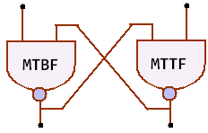
MTBF and MTTF can be distinguished
in two different
ways. 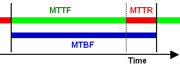
As shown in
the picture, MTBF is just MTTF + MTTR (mean time to repair). Instead of
repair, it could
also be
replacement, replenishment etc. Since this doesn't make any
difference, we just call it downtime. The key is that MTBF
includes downtime, but MTTF does not.
For most items the MTTR is quite small
compared to MTTF,
therefore MTTF ~ MTBF. However, the bigger and more comprehensive
the item is, the more different MTBF and MTTF get. For
example,
production lines and aircrafts consist of many piece parts, leading
to rather low MTBF and rather high downtime, therefore MTBF and
MTTF may differ substantially.
Because MTBF ~ MTTF in most cases, industries have
adopted either one or the other term for the same meaning. While
functional safety engineers tend to MTTF, logistics and maintenance
personnel prefer MTBF.
The
second way to distinguish MTTF from MTBF is not very common, but
nonetheless important. It can be
mathematically shown that for redundant / fault tolerant systems,
the mean time to first failure (then called MTTF) is different from the
mean time between failures (MTBF) in steady state. The distinction
between MTTF and MTBF becomes really important here, in particular when
the useful product life can be associated with either the "setting
time"
(characterized by MTTF), or the steady state (characterized by MTBF).
From now on we
will use only the term MTBF.
Up
|
3. MTBF simple and concise
|
Down
|
Let's begin with a simple example.
It will soon turn out that it is actually difficult, and, even
worse, it will raise a couple of questions that need comprehensive
answers.
- Let a population of the size of 100.000 units be 24 hours in
operation.
- --> During 24 h, 100.000 x 24 h = 2,4 million operating
hours will be cumulated.
- 2 failures have occurred.
What is the
best estimate for the MTBF of the population?  Most engineers would do the kind of calculation shown in the picture:
2,4 million operating hours / 2 failures = 1,2 million hours. If you
are a CEO or any other decision maker, you are allowed to stop reading
at this point as long as you take the warning to your heart: This math
is definitely wrong, and the bad thing is that it produces optimistic
MTBF figures! The correct figure is substantially
smaller than 1,2 million hours!
Most engineers would do the kind of calculation shown in the picture:
2,4 million operating hours / 2 failures = 1,2 million hours. If you
are a CEO or any other decision maker, you are allowed to stop reading
at this point as long as you take the warning to your heart: This math
is definitely wrong, and the bad thing is that it produces optimistic
MTBF figures! The correct figure is substantially
smaller than 1,2 million hours!
For the statisticians among you readers: The problem is not
statistical confidence or interval estimation.
OK, there are
a couple of questions begging for answers. The most difficult question
comes last.
- The correct MTBF calculation works quite different, and would
yield circa 900.000 hours,
which is
about 100 years. This is obviously not what we consider a
time, because no technical product would last 100 years without
failure.
Thus, MTBF is not a duration or a calendar time, but a parameter
characterizing the statistical failure behavior of the population of
units.
- The example has no information about the following:
- how long have the units already been in operation?
- what's the intended useful lifetime of the product?
10 to 20 years would be typical product lifetimes. On
the other hand, MTBF figures principally have no hard upper limit. One
to
10 million hours is pretty normal, and even a billion hours or more is
encountered quite often. Therefore, just concluding from the figures,
it seems clear that MTBF
and Lifetime must be different things.
- Is there any connection at all between MTBF and lifetime?
- The example also has no information about this:
- when
did the two failures occur?
For example, there is nothing wrong with the
assumption
that both failures could have occurred within the first 4 hours, with
no additional failure during the last 20 hours.
Or the first failure could have occurred in the first minute, and the
second failure in the last minute. The fact that no such information is
given implies that failures may occur arbitrarily at any time point.
- What's the nature of the failures are we talking about?
- As already mentioned, the calculation as shown above produces
optimistic results, and this is not a matter of statistical
confidence. Why is this, and
- why is it wrong to calculate MTBF just with simple math (rule
of three)?
 It is
difficult to answer any of these 4 questions
thoroughly without using answers from the other topics,
so please be patient and try to read through until the end of this
page.
It is
difficult to answer any of these 4 questions
thoroughly without using answers from the other topics,
so please be patient and try to read through until the end of this
page.
4.
MTBF misconceptions
Up
|
4.1
What does MTBF really mean and what's the purpose
|
Down
|
MTBF
is a simple and intuitive measure for the frequency of failures of
a given number of units operated at given ambient conditions. The
operator can easily estimate from the MTBF figure cost of labor and
spares associated with failures expected in the future. Thus, MTBF can
serve as an input parameter for operational planning.
 Systems
with many potential failure modes will fail more often than systems
with less failure modes, all other conditions being equal. Complex
systems naturally have many piece parts, and therefore more potential
failure modes than simple systems with less piece parts. For example, a
production line will fail more often than a hand drill.
Systems
with many potential failure modes will fail more often than systems
with less failure modes, all other conditions being equal. Complex
systems naturally have many piece parts, and therefore more potential
failure modes than simple systems with less piece parts. For example, a
production line will fail more often than a hand drill.
We can summarize the above in a more general way as follows:
All remaining circumstances being equal: The more piece parts needed
for operation, the more potential failure modes will be induced.
Therefore, more failures will actually happen, finally resulting in
lower MTBF. The same put much simpler:
More piece parts -->
lower MTBF
Less piece parts
--> higher MTBF
It is not too exaggerated if we consider MTBF as a measure of
complexity
in disguise of a reliability metric.
All following statements are equal:
- The MTBF is 1,2 million hours
- The failure rate is 0,833
failures per million hours
- The probability of failure is
8,33E-7 per hour
- The failure rate is 0,73 % per
year ("annual failure rate")

As mentioned before, the true MTBF figure of our example, namely circa
900.000 h (~100 years), cannot be considered a duration or a calendar
time, because this is much longer than any technical unit can be in
operation without failure. Therefore it is obvious that MTBF can not be
applied to a certain unit in a reasonable way.
However, if applied to a population of units, it suddenly makes sense
because a population of units would provide a substantial amount of
operating time during a relatively short calendar
time. In our example, 100.000 units provide altogether 2,4 million
operating hours in a single day!
Summarizing the above:
MTBF is a
simple and intuitive reliability measure for a
population of units.
This leads us to the next topic.
Here is a key
statement (will be explained
later):
- During its 10-year design life, the MTBF of the population of
units is 100 years
This
statement remains true if we replace "design life" with "life time",
"useful product life time", or any other kind of calendar time. This is
just a matter of interpretation and context.
The so-called bathtub
curve model, commonly used in quality management, explains
the
difference between MTBF and life time quite well.
The bathtub curve however shows the failure rate lambda instead of
MTBF. This is not just for the purpose of
looking like a bathtub, but because the calculation is easier with
failure rates than with MTBF. (The failure rate is simply the
reciprocal of MTBF)
The bathtub curve shows the
failure rate over time for a population of units. It shows 3
clearly distinguishable phases, which makes it an idealized model. In
real life, not every
phase would manifest in every case, and phases would sometimes overlap.
Phase
1:
At the beginning of the
product life, when units are put into operation, the failure rate may
be higher than originally expected. Suppliers typically react by fixing
(certain or selected) causes of failure, or by improving the product
quality in general. As a result, the failure rate becomes smaller over
time.
The characteristic of this phase is the decreasing failure rate (=
increasing
MTBF).
The failures in this phase
are called early failures, and the phase is often called early failure
phase or infant mortality phase.
|
 |
At
some point in time the supplier will decide that the product quality is
sufficiently good, and will therefore stop the quality improvement
process. The failure rate then will not decrease any more, instead it
will
turn into a kind
of steady state (constant failure rate over time), which
is the characteristic of this phase.
Constant failure rate over
time has strong implications, which are explained later in detail. |
 |
Finally,
when the useful product life is over, the product may
encounter an increasing failure rate
because of aging, wear-out, neglect of maintenance, etc.
The characteristic of
this phase is the increasing failure
rate (= decreasing
MTBF).
|
|
The
bathtub curve visualizes the
difference between MTBF and lifetime quite clearly. The next two pictures may
emphasize this a bit:
Lifetime is measured on the horizontal X-axis, representing a duration
or a calendar time, whereas MTBF (or 1/MTBF) is measured on the
vertical y-Axis, representing a parameter value of the
population of units.
The bathtub curve suggests that
1/MTBF is a kind of probability of failure of a product during its
whole lifetime.
The key
statement from the beginning of this paragraph puts it precisely:
- During its 10-year design life,
the MTBF of the population of units is 100 years
Careful readers may have
noticed that MTBF and lifetime may be indeed different, but there may
still
be some kind of (probably hidden) relationship between the two. Our example has been designed
with the purpose of avoiding any relationship. Remember: 100.000 units
have been operated for 24 hours with 2 failures. There is no mention of
Lifetime at all.
hidden) relationship between the two. Our example has been designed
with the purpose of avoiding any relationship. Remember: 100.000 units
have been operated for 24 hours with 2 failures. There is no mention of
Lifetime at all.
Now let's introduce lifetime into our example. Let 20 units be 10 years
24/7 in operation, with altogether 2 failures. This is 200 cumulative
operating years, with 2 failures, and again we obtain circa 100 years
MTBF by doing simple math (which is, as clearly emphasized before,
wrong. The
correct figure is 75 years. More on this later).
Just by modifying our example,
the probability nature of MTBF becomes more obvious: 200 units have
been operated for a lifetime, and 2 have failed. --> The probability
of failure of a unit during its lifetime seems to be 2/200 = 1%.
 Let's
modify our example again by substantially increasing the complexity:
Trucks and cars for example are quite likely to
fail at least once in their lifetime. Aircrafts typically fail once
every month (which has no worse impact due to their redundant design),
and production lines even tend to fail every hour. The MTBF for these
items is either comparable to their lifetime (cars, trucks),
or may be even lower (aircrafts, production lines).
Let's
modify our example again by substantially increasing the complexity:
Trucks and cars for example are quite likely to
fail at least once in their lifetime. Aircrafts typically fail once
every month (which has no worse impact due to their redundant design),
and production lines even tend to fail every hour. The MTBF for these
items is either comparable to their lifetime (cars, trucks),
or may be even lower (aircrafts, production lines).
In contrast to what we stated above, namely that MTBF cannot be applied
to single units in a useful way, it seems that if only the items
are sufficiently complex, it definitely can, because then the
probability
of failure during lifetime is so high that the majority of the items
would encounter at least one failure.
Therefore, if MTBF
is sufficiently low compared to lifetime, which is true for
sufficiently complex units, MTBF can be applied to single units.
Up
|
4.3 Random
failures versus systematic failures
|
Down
|
 The
foundation of the MTBF model is the distinction between random failures
and
systematic failures. Random failures are unpredictable, and therefore
occur unexpectedly. In contrast, systematic failures are predictable,
and can therefore at least theoretically be avoided, if the operator
could and if budget would allow. The MTBF model requires that
systematic failures either
don't exist, or they can be considered negligible or disregarded for
other
(valid) reasons. "Constant failure rate" is the mathematical wording
for the absence of systematic failures, where failures occur only
randomly.
The
foundation of the MTBF model is the distinction between random failures
and
systematic failures. Random failures are unpredictable, and therefore
occur unexpectedly. In contrast, systematic failures are predictable,
and can therefore at least theoretically be avoided, if the operator
could and if budget would allow. The MTBF model requires that
systematic failures either
don't exist, or they can be considered negligible or disregarded for
other
(valid) reasons. "Constant failure rate" is the mathematical wording
for the absence of systematic failures, where failures occur only
randomly.
Chance
means that things evolve in a way we cannot predict. More
precisely: The Inability to predict the point of time of a failure
event. The reason for this inability is not just missing knowledge or
experience, but rather the fact that the necessary knowledge doesn't
even exist, because the laws of nature literally don't allow its
existence. It is not a technological issue, nor is it a lack of
technological progress that prevents us from obtaining this knowledge.
Even worse, we already do know since decades of the existence of
events, for which nature doesn't offer the kind of information we would
need for prediction. In science, these types of events are
called random events, which emphasizes that objective randomness in
fact
exists. We see real randomness for example in:
- radioactive decay of isotopes
(it is impossible to predict the point in time of the decay of a
certain atom), or
- cell division (it is impossible to predict the point in
time of the next division of a certain biological cell)
Real
randomness has a sound foundation in theoretical physics. The so-called
bell inequality is the proof that real (or objective)
randomness exists, and, moreover, randomness is nothing less than "the
driving force" of nature.
Now let's go back to our MTBF context. We already know that objectively
random events, and therefore unpredictable failure events exist. But
what are random technical failures exactly? Let's answer this first
from the natural science viewpoint. The functioning of electronic
equipment comes down to the behavior and effects of electrons in atoms
and crystals. We know that it is difficult, if not impossible, to
explain effects on microcosmic scale with the
same natural laws we apply to macroscopic scale. Therefore, quantum
mechanics was "invented", which, despite
all its peculiarities, perfectly explains the world on microcosmic
scale. We know from quantum mechanics, that on microscopic scale a lot
of things are going on just for no reason, continually producing random
events. Some events kind of evolve or propagate in such a way that
their effects become noticeable on larger scale, where they manifest
as random, macroscopic events.
The question is: Is this what the MTBF model and the bathtub curve mean
by random failures? No, because these events (microscopic random events
noticeably manifesting on macroscopic scale) are so rare that they're
quantitatively irrelevant. Nevertheless is it important to
understand that randomness is not just an excuse for (human) technical
inability, but a real and objective thing that constitutes
nature.

Let the company design and manufacture a product. The product is
introduced into the market, but the product somehow encounters more
failures than expected. The defect units are sent back to the company
where the quality management (QM) department scrutinizes them for the
causes of failure. Let's assume that the QM finds the cause for 70% of
all defects. The company's corrective action procedures lead to design
changes, and finally these defects get fixed.
- Note that 70% have been fixed
just by using established processes and personnel doing their routine
jobs.
Later
on, either the market or the company's management conclude that
70&
is not enough. Therefore a task force is initiated, which is able to
find causes for another 20% of failures.
- Note that another 20% could be
fixed, however with additional effort (time and budget)
Later on, 90%
is still considered not good enough, therefore the company approaches
an external laboratory, which is able to
find causes for another 9% of failures. Now, in addition to 90% of all
failures already fixed, another 9% is well understood. It turns out
that, despite of understanding the cause, it is either too
expensive for the company, or the company doesn't have the necessary knowledge for a
fix. The management finally decides that fixing 4%
would be a reasonable match with time and budget the company can
afford, while the remaining 5% will remain unfixed.
We know that
in theory our company could at least fix 99% of all causes if only
enough budget was available.
Also, if the company had approached an even better / more experienced
laboratory, or many laboratories instead of only one, maybe all
100% of causes could have been identified, and, with unlimited budget
available, all of them could be fixed.
But
this would be possible only in a world driven by natural laws only.
But in our company's world, economic and other rules also play
important roles, and there, 94% is the end of the road. May be for a
different company, 98% would be the end of the road. Or 85%, or
... ..
The
point is that even the company could do more technically, it couldn't
do more economically, and therefore, the remaining 6% of failures will
continue to "just happen" = occur randomly.
We can draw
this even further:
- Our
company (A) tries to fix all failures it can. It can fix 94%, knows the
cause of another 5% but can't fix, and has no clue about the remaining
1%.
Let's suppose competitive companies with the same product:
- Company B fixing 94%, but has
no clue of the remaining 6%.
- Company C understanding all
100% of causes and being able to fix 100%, but fixing only 94%.
Does this make
any difference? No, because customers wouldn't see any difference.
--> It makes no difference for the MTBF model if companies cannot fix failures, or don't want to fix failures.
Summary:
- The MTBF model requires that only
unpredictable = random failures exist.
- Randomness
is the driving force of nature on microscopic scale, but it is very
rare that microscopic random events manifest on macroscopic scale.
- The
distinction between random failures and systematic failures depends on
what the company can/cannot or wants / doesn't want to fix.
- Randomness
in economic context is mainly defined by what a company can accomplish
or wants to afford. If we understand time and budget constrains as laws
comparable and equivalent to natural laws, then the "border" to
randomness begins where the company's ability or will ends.
- One
of the reasons why the MTBF model is so badly understood (e.g.
confusion with life time) is the fact that randomness in this
context is always a mix between objective randomness, and the
ability or will of a company.
Key statement:
MTBF
considers only random events. What is random and what is not,
depends
on ability and will, and therefore on the "statistical distance" of the
viewer.
Up
|
4.4 MTBF Calculation from Field Data
|
Down
|
The
following information is tailored to field data, but it can also be
applied to any other failure data, for example laboratory test data.
Up
|
4.4.1 Simple but excellent MTBF Approximation
Formula
|
Down
|
Recap of our MTBF example from
above:
- 100.000 units have been 24
hours in operation. --> 2,4 million operating hours have been
cumulated.
- There were altogether 2 failures
It seems to be
a no-brainer to calculate MTBF by dividing the cumulative operating
hours by the # of fails, but this is terribly wrong, and, even worse,
it produces optimistic results.
 Before we show
the correct calculation method, we first offer a simple but extremely
good approximation, which
produces slightly pessimistic results. In worst case it is 1%
pessimistic. For example, if the correct result was 1.000 h, the
approximation would yield some figure between 990 h and 1000 h.
The diagram
below shows in detail the quality of the approximation for data sets
with 0
to 20 failures.
Before we show
the correct calculation method, we first offer a simple but extremely
good approximation, which
produces slightly pessimistic results. In worst case it is 1%
pessimistic. For example, if the correct result was 1.000 h, the
approximation would yield some figure between 990 h and 1000 h.
The diagram
below shows in detail the quality of the approximation for data sets
with 0
to 20 failures.
- Example 1: In the diagram we read 99,5% for n=4 failures. This
means, for example, if the correct MTBF were1.000 hours, the
approximation would yield 995 hours.
- Example
2: The diagram shows 99% for n = 1 failure. If the correct MTBF were
1.000 hours, the approximation would yield 990 hours. This is the worst
case (1% pessimistic)
- Example 3: For the most
interesting case, n = 0 failures, the diagram tells us 99,7%.
Therefore, if the correct MTBF were 1.000 hours, the approximation
would
yield 997 hours.
More
details on this can be found later in the next but one paragraph, and
even more details can be found in my MTBF script (unfortunately available only in
German).
Up
|
4.4.2
How randomness affects MTBF calculation
|
Down
|
For the zero
failure case it is clear that MTBF cannot be calculated with simple
math, because division by zero would yield infinitely high MTBF
figures. On the other hand, if the amount of cumulative
operating hours is not infinitely high, there must be some MTBF figure,
and therefore a valid calculation method should exist accordingly.
Here is the fallacy:
The simple math approach ignores the random nature of the failure
events. The following illustrations hopefully explain what this means.
- A man on
a sightseeing trip reaches a bus stop. Unfortunately there is no
timetable, but the man knows that every
full hour a bus would stop. His wristwatch tells him the current time,
and finally he
can conclude how long he has to wait for the next bus.
- Same scenario as 1., with the only difference that the man has no
access to a watch. He doesn't know the actual time, but he
knows that the bus stops every (full) hour.
Conclusion: The man must wait 30 minutes on average.
- Same scenario as 2., with the following difference: The bus comes
randomly, and the average time between two stops is one hour. Just to
make it clear: The only difference is that we replaced the "timetable
property" by randomness. The bus now comes at random points in time,
but on average it takes one hour between two stops. The mathematical
expression goes like this: The bus arrivals are exponentially
distributed with average 1 hour.
How long must the man wait - on average- when he arrives at the bus
stop? One hour.
Let's draw this further:
- Same scenario as 3., with the following difference: When the man
arrives at the bus stop, another man is already waiting, and tells him
that the last bus was 2 hours ago.
In this scenario, the bus still comes every hour (on average), but the
last stop was already 2 hours ago.
Is this any different from scenario 3? No, because the information
"last stop already 2 hours ago" is just a manifestation of randomness,
and the information that it is random, is already given. Therefore the
information about the last bus is useless, and the man must wait one hour on average.
The principle behind scenario 4. may be easier to realize if we put it
like this:
An ideal dice has been cast 30 times with no six. What's the
probability of a six in the next cast? --> p = 1/6. The
information "30 times with no six" is
irrelevant because the information "ideal dice" is given.
Lottery makes it really apparent that this is difficult to grasp, since
many people believe that numbers (not) drawn in the past has any effect
on future drawings.
Scenarios 3.
and 4. are absolutely relevant for the MTBF model, whereas 1. and 2.
are not.
Randomness somehow challenges the human brain. Random events occur
arbitrarily,
and are therefore impossible to predict. In a random event
scenario, the occurrence of the next event has no relationship with the
occurrence of past events. More generally put: The event history is
meaningless for the next event.
Key statement:
In
a random event scenario, the points in time of events are
unpredictable, regardless how much we know about past events. The event
frequency
is the only
information we can obtain from past events.
Future events, of course, will occur with that frequency, provided
that all other conditions remain equal.
There are a couple of consequences arising of this, but here we present
only one, because otherwise it would go too far:
By applying the MTBF model to a population of units, we say that
failure events occur randomly. The only information we can obtain from
past failure events is the failure frequency. That past frequency will
be the future frequency. The frequency is the only thing we know,
therefore the future behavior of the population of units will be the
same like the past behavior. This is true regardless of the duration of
the past, or more precisely, regardless of how long the units
have already been in operation. This finally means that in the MTBF
model the units
are "ageless", and in particular, every unit can be considered new,
regardless of the operating time they may already have cumulated.
There are more interesting consequences.
These are described in my MTBF script, which is available only
in German.
Up
|
4.4.3. Exact MTBF Calculation Formula
|
Down
|
Some general
math first:
- The poisson distribution describes
how many random events will occur in a given
timeframe.
We would use it to calculate this:
- How many failure events
- will occur in the next x hours,
- and what's the probability for this
Examples:
- The probability that we see not more than 2 failures in the
next 100 hours is 90%.
- The probability that we see not more than 3 failures in the
next 100 hours is 95%.
- The probability that we see at least 1 failure in the next
100 hours is 30%.
- The probability that we see exactly 2 failures in the next
100 hours is 5%.
- We obtain the gamma distribution
by integrating the poisson over time.
The Gammak describes how
long it takes for k random events
to occur.
We would use it to calculate this:
- How long will it take
- for y events to occur,
- and what's the probability for this
Examples:
- The probability that the next 2 failures take no longer than
200 hours is 90%.
- The probability that the next 3 failures take no longer than
300 hours is 95%.
- The probability that the next 3 failures take at least 300
hours is 5%.
- The Gammak
is the k-fold convolution of the exponential distribution.
--> The Exponential describes how
long it takes for one random event
to occur.
- The Chi Square distribution
doesn't describe natural processes, but is rather a kind of man-made
distribution, designed for a certain statistical purpose. The Chi
Square is and
has ever been one of the three statistical distributions, which
have been available in tabulated form in the early days before software
and pocket calculators existed.
This was even more practical
because, simply speaking, all statistical distributions can be
transformed into these three distributions.
In particular, the Gamma can
be expressed with the Chi Square, and finally the correct formula to
calculate MTBF from field data is:
where n is the # of failures,
and alpha the statistical confidence level. If you're not interested in
statistical confidence, then use alpha = 50% (mathematically speaking =
point estimation). Readers may get an Excel template on
request.
More
details can be found in my MTBF script, which is available only
in German.
Up
|
5. MTBF calculation according to
established Standards
|
To top
|
Direct link to
MTBF calculation standards.
Field
data, if obtained properly, is by far the best data source for MTBF,
and even incomplete or even flawed field data is often still better
than other data sources. The reason is that the failure information
contained in field data comes from units exposed to real operating
conditions in real environments, exposed to the behavior of real
users. By using failure data, the probability of covering everything
that could affect MTBF is higher than with any other data source.
However, there are two general
issues with field failure data, with opposite effect:
- Field failure data often contains findings that are not
necesarily attributable to the units under investigation, and
therefore not relevant for MTBF. User misunderstanding, user errors,
operation outside specification and the like isn't negligible in most
cases.
- This issue alone would decrease the calculated MTBF
- The failure feedback process from the field may have issues.
Maybe there is only an informal feedback process.
But even despite established feedback process, MTBF relevant findings
may still not (or insufficiently) be reported, because maintenance /
repair technicians under time pressure try to get the system back into
operation as fast as they can, rather than dealing with stupid feedback
forms.
While some
companies never get information at all about how their products fare in
the field, the majority of companies is able to get at least some
feedback. Typically they don't have established feedback processes, but
they somehow manage to derive usable MTBF-relevant information from
other processes.
Some companies have established
field data collection and evaluation processes (like FRACAS, failure
reporting and corrective action system), but only a few of them are
designed for delivering sufficiently
eligible data in order to obtain reliable MTBF figures. The last
sentence clearly means that well-established field data collection
and evaluation process are not necessarily a guarantee for reliable
MTBF figures, because such processes must be specifically designed for
this purpose.
Established
international MTBF calculation standards can
be conceived as sets of empiric formulas, derived from comprehensive
field failure data that have been collected over many years. Only big
companies and governmental organizations can stem such efforts, for
example:
- Siemens company (SN 29500)
- Bellcore, later Telcordia, now
Ericsson (Telcordia SR-332)
- British telecom (HRD5)
- A consortium of the French
industry (FIDES)
- The US department of defense
(Mil-HDBK-217)
- A consortium of the Chinese industry (GJB/Z 299)
All
these standards have one thing "in common": They produce very different
MTBF figures for the same system / component under the same
environmental conditions.
In order to explain why, we first
repeat a key statement from further above, followed by other possible
reasons:
- MTBF considers only random events. What is
random and what is not,
depends on ability and will, and therefore
on the "statistical distance" of the viewer.
- Telecom
equipment and military equipment have completely different use cases
and failure causes. Moreover, the exposure of telecom technicians and
soldiers to their equipment may differ substantially.
- It can make a big difference if
the entity that establishes the MTBF calculation standard is a customer
that buys equipment (the US department of defense), or a supplier
selling his equipment (Siemens and Telecom companies).
Next Topic

 Search
this site
Search
this site


